来自Uber H3:H3: Uber’s Hexagonal Hierarchical Spatial Index
最近一个项目用到了Uber这个H3六边形层级系统,用到了空间索引提升查询效率

Grid systems are critical to analyzing large spatial data sets, partitioning areas of the Earth into identifiable grid cells.
With this in mind, Uber developed H3, our grid system for efficiently optimizing ride pricing and dispatch, for visualizing and exploring spatial data. H3 enables us to analyze geographic information to set dynamic prices and make other decisions on a city-wide level. We use H3 as the grid system for analysis and optimization throughout our marketplaces. H3 was designed for this purpose, and led us to make some choices such as using hexagonal, hierarchical indexes.
Earlier this year, we open sourced H3 on Github, giving others access to this powerful solution, and last week, we open sourced our H3 JavaScript bindings. In this article, we discuss why we use a grid system, some of the unique properties of H3, and how you can get started using H3.
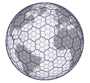
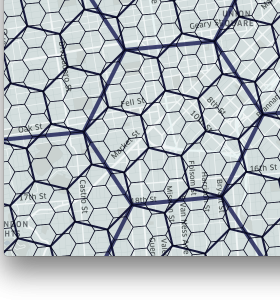
Figure 1. H3 enables users to partition the globe into hexagons for more accurate analysis.
Analysis using grids
Every day, millions of events occur in the Uber marketplace. Every minute, riders request rides, driver-partners start trips, and hungry users request food, among other actions on the platform. Each event happens at a specific location, for example, a rider requests a ride from home, and a driver accepts that request in their car just a few miles away.
These events empower Uber to better understand and optimize the marketplace for users across our services. For instance, these events might tell us that there is more demand than supply in a certain part of a city and adjust pricing in response, or inform the platform that there are two ride requests within close proximity to a specific driver on uberPOOL.
Deriving information and insights from data in the Uber marketplace requires analyzing data across an entire city. Because cities are geographically diverse, this analysis needs to happen at a fine granularity. Analysis at the finest granularity, the exact location where an event happens, is very difficult and expensive. Analysis on areas, such as neighborhoods within a city, is much more practical.
 |
 |
 |
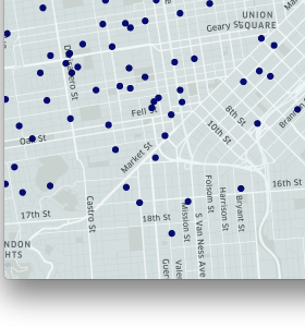
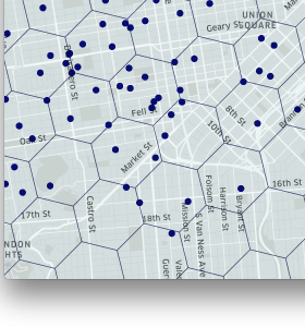
| Figure 2. The maps above depict the process of bucketing points with H3: cars in a city; cars in hexagons; and hexagons shaded by number of cars. |
We use a grid system to bucket events into hexagonal areas, in other words, cells. Data points are bucketed into hexagons and can be written using the hexagonally bucketed data. For example, we calculate surge pricing by measuring supply and demand in hexagons in each city that we serve. These hexagons form the basis for our analysis of the Uber marketplace.
Hexagons were an important choice because people in a city are often in motion, and hexagons minimize the quantization error introduced when users move through a city. Hexagons also allow us to approximate radiuses easily, such as in this example using Elasticsearch.
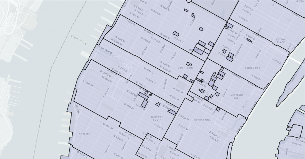
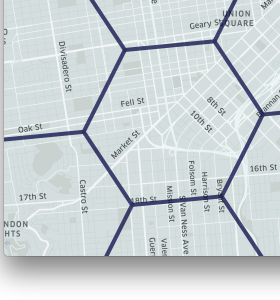
Figure 3. Zip code map of New York City (Manhattan).
There are other choices we could use for bucketing events into areas, for instance polygonal zones around areas. These could be postal code areas, but such areas have unusual shapes and sizes which are not helpful for analysis, and are subject to change for reasons entirely unrelated to what we would use them for. Zones could also be drawn by Uber operations teams based on their knowledge of the city, but such zones require frequent updating as cities change and often define the edges of areas arbitrarily.
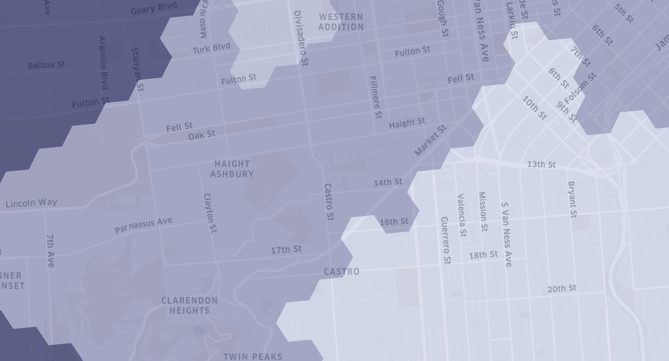
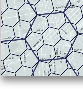
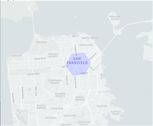
Figure 4. Randomly generated hexagonal clusters cover the city of San Francisco.
Grid systems can have comparable shapes and sizes across the cities that Uber operates in and are not subject to arbitrary changes. While grid systems do not align to streets and neighborhoods in cities, they can be used to efficiently represent neighborhoods by clustering grid cells. Clustering can be done using objective functions, producing shapes much more useful for analysis. Determining membership of a cluster is as efficient as a set lookup operation.
H3
We decided to create H3 to combine the benefits of a hexagonal global grid system with a hierarchical indexing system.
A global grid system usually requires at least two things: a map projection and a grid laid on top of the map. A map projection is needed for going from a three-dimensional location on Earth to a two dimensional point on a map. A grid is then overlaid on the map, forming a global grid system.
This process can be accomplished in innumerable ways by combining different map projections and grids, for example, the widely recognized Mercator projection and a square grid. While this simple method would work, it has a number of drawbacks. To start, the Mercator projection has significant size distortion, so some cells will have vastly different areas. Square grids also have drawbacks, requiring multiple sets of coefficients when used for analysis. This disadvantage is a result of squares having two different types of neighbors, one type with which they share an edge (in the four cardinal directions) and another type with which they share a vertex (in four diagonal directions).
 |
 |
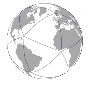 |
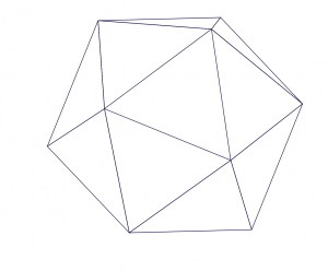
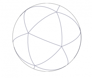
| Figure 5. We chose to use gnomonic projections centered on icosahedron faces (left) for H3’s map projection, projecting Earth as a spherical icosahedron (right). |
For map projection, we chose to use gnomonic projections centered on icosahedronfaces. This projects from Earth as a sphere to an icosahedron, a twenty-sided platonic solid. An icosahedron-based map projection results in twenty separate two-dimensional planes rather than a single plane. The icosahedron can be unfolded in many ways, producing a two-dimensional map each time. H3, however, does not unfold the icosahedron to build its grid system, and instead lays its grid out on the icosahedron faces themselves, forming a geodesic discrete global grid system.
 |
 |
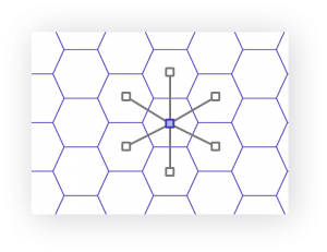 |
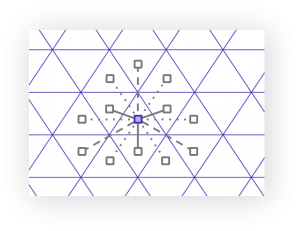
| Figure 6. Distances from a triangle to its neighbors (left), a square to its neighbors (center), and a hexagon to its neighbors (right). |
Using a hexagon as the cell shape is critical for H3. As depicted in Figure 6, hexagons have only one distance between a hexagon centerpoint and its neighbors’, compared to two distances for squares or three distances for triangles. This property greatly simplifies performing analysis and smoothing over gradients.

Figure 7. H3 used to create a grid on a single icosahedron face.
The H3 grid is constructed by laying out 122 base cells over the Earth, with ten cells per face. Some cells are contained by more than one face. Since it is not possible to tile the icosahedron with only hexagons, we chose to introduce twelve pentagons, one at each of the icosahedron vertices. These vertices were positioned using the spherical icosahedron orientation by R. Buckminster Fuller, which places all the vertices in the water. This helps avoid pentagons surfacing in our work.
 |
 |
 |
| Figure 8. H3 enables the user to subdivide areas into smaller and smaller hexagons. |
H3 supports sixteen resolutions. Each finer resolution has cells with one seventh the area of the coarser resolution. Hexagons cannot be perfectly subdivided into seven hexagons, so the finer cells are only approximately contained within a parent cell.
The identifiers for these child cells can be easily truncated to find their ancestor cell at a coarser resolution, enabling efficient indexing. Because the children cells are only approximately contained, the truncation process produces a fixed amount of shape distortion. This distortion is only present when performing truncation of a cell identifier; when indexing locations at a specific resolution, the cell boundaries are exact.
Getting started with H3
The H3 indexing system is open source and available on GitHub. The H3 libraryitself is written in C, and bindings are available for a number of languages. Using bindings is the recommended way to start using H3. Uber has published bindings for Java and JavaScript, and the community has contributed bindings for more languages. Bindings are coming soon for Python and Go.
 |
 |
 |
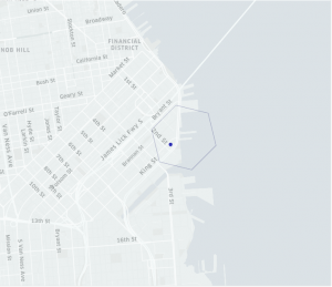
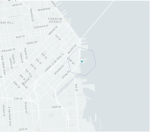
| Figure 9. The point (blue, left) and its containing hexagon, the centroid (lighter blue, middle) of its containing hexagon, and both the point and centroid of the containing hexagon (right) depict a possible difference between the two. |
Code: https://github.com/uber/h3/blob/master/examples/index.c
The basic functions of the H3 library are for indexing locations, which transforms latitude and longitude pairs to a 64-bit H3 index, identifying a grid cell. The function geoToH3 takes a latitude, longitude, and resolution (between 0 and 15, with 0 being coarsest and 15 being finest), and returns an index. h3ToGeo and h3ToGeoBoundary are the inverse of this function, providing the center coordinates and outline of the grid cell specified by the H3 index, respectively.
Once you have data indexed using H3, the H3 API has functions for working with indexes.
 |
 |
 |
| Figure 10. Hexagons neighboring an index, with distance of 0 (left; just the original index), 1 (middle; with neighbors of the original index), and 2 (right; with neighbors of neighbors). |
Code: https://github.com/uber/h3/blob/master/examples/neighbors.c
Neighboring hexagons have the useful property of approximating circles using the grid system. The kRing function provides grid cells within grid distance k of an origin index.
 |
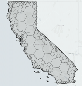 |
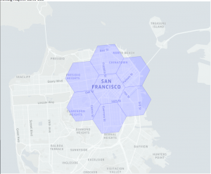
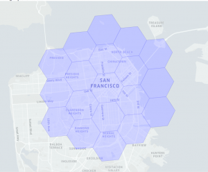
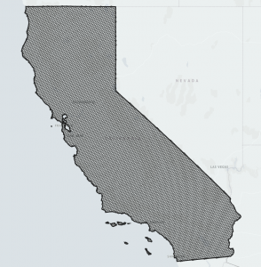
| Figure 11. Dense hexagons representing California stand in stark contrast to compact hexagons representing the state, requiring many fewer hexagons to represent the same area. |
Code: https://github.com/uber/h3/blob/master/examples/compact.c
The hierarchical nature of H3 allows for efficiently truncating the precision (or resolution) of an index and recovering the original indexes. The uncompact and compact representations of a set of hexagons are shown above. The uncompact representation has 10,633 hexagons at resolution 6, but the compact representation has 901 hexagons at resolutions up to 6. In both cases, a hexagon index is a 64-bit integer.
The precision of a single index can also be efficiently truncated as a bitwise operation, or expanded to a higher precision set of indexes.
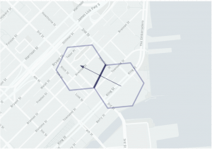
Figure 12. H3 can represent the movement from one cell to another, here represented by drawing an arrow from the origin to destination cell.
Code: https://github.com/uber/h3/blob/master/examples/edge.c
H3 has functions for directed edges of grid cells which can represent the movement from one cell to another. Directed edges can be stored as 64-bit integers, and can be obtained from two neighboring cells, or by finding all edges of a cell. When needed, an edge can be converted back to the origin or destination indexes.
Moving forward
H3 is used throughout Uber to support quantitative analysis of our marketplace, and now that it’s open sourced, you too can hexagonify the world! We look forward to you joining the H3 community by following our repository on Github and tweeting with the #uberH3 hashtag.
Maps generated using MapboxGL.
Learn more information about our mapping data providers.
Major contributors to the H3 library also include Kevin Sahr (Southern Oregon University), Joseph Gilley (Uber), Nick Rabinowitz (Uber), and David Ellis (CarDash).
Subscribe to our newsletter to keep up with the latest innovations from Uber Engineering.
